The partial derivatives of a function with several independent variables are those obtained by taking the ordinary derivative in one of the variables, while the others are maintained or taken as constants.
The partial derivative in one of the variables determines how the function varies at each point, per unit of change in the variable in question.
By its definition, the partial derivative is calculated by taking the mathematical limit of the quotient between the variation of the function and the variation of the variable with respect to which it is derived, when the change of the latter tends to zero.
Suppose the case of a function f that depends on the variables x and y , that is, for each pair (x, y) a z is assigned :
f: (x,y) → z .
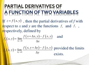
The partial derivative of the function z = f(x, y), with respect to x is defined as:
![]()
Now, there are several ways to denote the partial derivative of a function, for example:
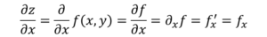
The difference with the ordinary derivative, in terms of notation, is that the d of the derivative is changed to the symbol ∂, known as “Jacobi’s D”.
Properties of partial derivatives
The partial derivative of a function of several variables, with respect to one of them, is the ordinary derivative in said variable and considering the rest as fixed or constant. To find the partial derivative, the rules for the differentiation of ordinary derivatives can be used.
Below are the main properties:
Continuity
If a function f(x, y) has partial derivatives at x and y at the point (xo, yo) then the function can be said to be continuous at that point.
Chain rule
A function f(x,y) with continuous partial derivatives on x and y, which in turn depends on a parameter t through x=x(t) and y=y(t) , has an ordinary derivative with respect to the variable t , which is calculated using the chain rule:
dt z = ∂xz dtx + ∂yz dty
Closing or lock property
The partial derivative with respect to one of the variables of a function f of two or more variables (x, y, …) , is another function g in those same variables, for example:
g(x, y, …) = ∂y f(x, y, …)
That is, partial differentiation is an operation that goes from R n to R n . In that sense it is said to be a closed operation .
Successive partial derivatives
Successive partial derivatives of a function of several variables can be defined, giving rise to new functions on the same independent variables.
Let the function be f(x,y). The following successive derivatives can be defined:
fxx = ∂xf ; fyy = ∂yyf ; fxy = ∂xyf y fyx = ∂yxf
The last two are known as mixed derivatives because they involve two different independent variables.
Schwarz theorem
Let be a function f(x,y), defined in such a way that its partial derivatives are continuous functions on an open subset of R 2 .
Then, for each and every pair (x, y) that belongs to said subset, we have that the mixed derivatives are identical:
∂xyf = ∂yxf
The above statement is known as Schwarz’s theorem .
How are partial derivatives calculated?
Partial derivatives are calculated in a similar way to ordinary derivatives of functions in a single independent variable. When the partial derivative of a function of several variables is taken with respect to one of them, the other variables are taken as constants.
Several examples are given below:
Example 1
Let the function be:
f(x,y) = -3x2 + 2(y – 3)2
We are asked to calculate the first partial derivative with respect to x and the first partial derivative with respect to y .
Procedure
To calculate the partial of f with respect to x , take y as a constant:
∂xf = ∂x( -3x2 + 2(y – 3)2 ) = ∂x( -3x2 )+ ∂x( 2(y – 3)2 ) = -3 ∂x(x2) + 0 = -6x.
And in turn, to calculate the derivative with respect to y , x is taken as a constant:
∂yf = ∂y( -3x2 + 2(y – 3)2 ) = ∂y( -3x2 )+ ∂y( 2(y – 3)2 ) = 0 + 2·2(y – 3) = 4y – 12.
Example 2
Determine the second-order partial derivatives: ∂ xx f, ∂ yy f, ∂ yx f and ∂ xy f for the same function f of example 1.
Procedure
In this case, since the first partial derivative in x and y is already calculated (see example 1):
∂ xx f = ∂ x (∂ x f) = ∂ x (-6x) = -6
∂yyf = ∂y(∂yf) = ∂y(4y – 12) = 4
∂ yx f = ∂ y (∂ x f) = ∂ y (-6x) = 0
∂xyf = ∂x(∂yf) = ∂x(4y – 12) = 0
It is observed that ∂ yx f = ∂ xy f , thus fulfilling Schwarz’s theorem, given that the function f and its first-order partial derivatives are all continuous functions in R 2 .
Solved exercises
Exercise 1
Let the function be:
f(x,y) = -x2 – y2 + 6
Find the functions g(x,y) = ∂ x f and h(x,y) = ∂ y f.
Solution
The partial derivative of f with respect to x is taken , for which the variable y is made constant:
g(x, y) = – 2x
In a similar way, the partial derivative of g with respect to y is taken , making x constant, resulting for the function h :
h(x, y) = -2y
Exercise 2
Evaluate for point (1, 2) the functions f(x, y) and g(x, y) from exercise 1. Interpret the results.
Solution
The values x=1 and y=2 are substituted , obtaining:
f(1,2) = -(1)2 -(2)2 + 6= -5 + 6 = 1
This is the value that function f takes when it is evaluated at that point.
The function f(x,y) is a two-dimensional surface and the coordinate z=f(x,y) is the height of the function for each pair (x,y) . When the pair (1,2) is taken , the height of the surface f(x,y) is z = 1.
The function g(x, y) = – 2x represents a plane in three-dimensional space whose equation is z = -2x or -2x + 0 and -z =0 .
Said plane is perpendicular to the xz plane and passes through the point (0, 0, 0) . When evaluated at x=1 and y=2 then z = -2 . Note that the value z=g(x,y) is independent of the value assigned to the variable y .
On the other hand, if the surface f(x, y) is intersected with the plane y= c, with c constant, we have a curve in the plane zx : z = -x 2 – c 2 + 6 .
In this case the derivative of z with respect to x coincides with the partial derivative of f(x,y) with respect to x : d x z = ∂ x f .
When evaluating the pair (x=1, y=2) the partial derivative at that point ∂ x f(1,2) is interpreted as the slope of the tangent line to the curve z= -x 2 + 2 at the point (x=1, y=2) and the value of said slope is -2.
